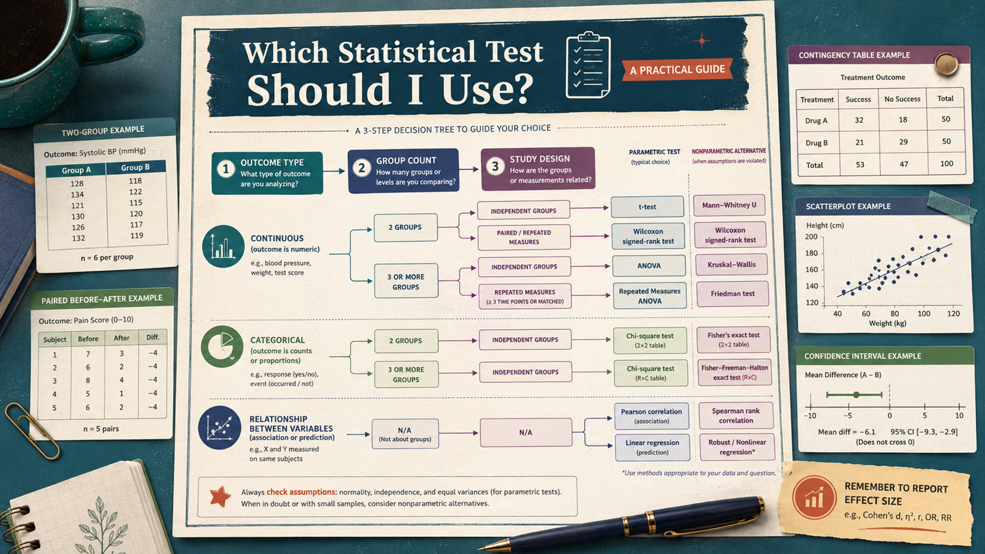
Which statistical test should I use? Start with the type of outcome you measured, not the name of your project. Then ask whether you are comparing groups or testing a relationship, how many groups or time points you have, and whether the observations are independent or paired.

For a continuous outcome, two independent groups usually point to a Welch independent-samples t-test. Two measurements from the same people point to a paired t-test. Three or more independent groups point to ANOVA, and three or more repeated measurements point to repeated-measures ANOVA or a mixed-effects model.

For categorical counts, think chi-square, Fisher’s exact test, McNemar’s test, or logistic regression. For relationships between numeric variables, think Pearson or Spearman correlation. For prediction or adjustment, think regression.

The test name is only the beginning. A defensible analysis also checks independence, data quality, assumptions, effect size, confidence intervals, missing data, multiple comparisons, and whether the study design can support the conclusion.

Statistical test decision tree branching from outcome type and study design to t-tests, ANOVA, chi-square, correlation, regression, and nonparametric alternatives

Quick answer: choose the test from the outcome and design

Your research question	Common test	Main alternative	Critical detail
Is one sample mean different from a known value?	One-sample t-test	One-sample Wilcoxon signed-rank or sign test	The benchmark and direction of the hypothesis should be defined before examining the result.
Is one observed proportion different from a benchmark?	Exact binomial test or one-sample proportion test	Confidence-interval-based analysis	Use the number of successes and total observations, not only the observed percentage.
Do two independent groups have different means?	Welch independent-samples t-test	Mann–Whitney U test	The people or units in one group must not also appear in the other group.
Did the same participants change from before to after?	Paired t-test	Wilcoxon signed-rank test	Analyze within-person differences rather than treating the measurements as independent groups.
Do three or more independent groups differ?	One-way ANOVA or Welch ANOVA	Kruskal–Wallis test	A significant omnibus result does not identify which groups differ.
Did the same participants complete three or more conditions?	Repeated-measures ANOVA	Friedman test or mixed-effects model	Repeated observations from the same participant are correlated.
Are two independent categorical variables associated?	Chi-square test of independence	Fisher’s exact test for a sparse 2×2 table	Enter observed counts, not percentages alone.
Did a paired yes/no outcome change from before to after?	McNemar’s test	Exact McNemar test for small discordant counts	Ordinary chi-square treats observations as independent and is not appropriate for paired binary data.
Are two continuous variables linearly related?	Pearson correlation	Spearman rank correlation	Correlation does not establish causation.
Do predictors explain a continuous outcome?	Linear regression	Robust, transformed, nonlinear, or mixed models	Inspect residuals and model form, not only coefficient p-values.
Do predictors explain a yes/no outcome?	Binary logistic regression	Other generalized linear or mixed models	Odds ratios are not automatically equivalent to risk ratios.
Are you pooling estimates from several studies?	Meta-analysis	Structured narrative synthesis	The unit of analysis is the study estimate, not an individual participant.

Fastest reliable rule: identify the outcome type first, then the study design. Do not choose a test because it produced the smallest p-value.

A practical statistical test decision tree

Answer these five questions in order. Most common analyses become clear by the fourth question.

Decision	Question to ask	If yes	If no
1. Define the outcome	Is the main outcome numeric and meaningfully measured on a scale?	Continue toward t-tests, ANOVA, correlation, or linear regression.	For categorical outcomes, continue toward binomial, chi-square, Fisher’s exact, McNemar, or logistic regression.
2. Define the purpose	Are you comparing groups or conditions?	Count the groups and decide whether observations are independent or paired.	If testing a relationship or prediction, use correlation or regression.
3. Count the groups	Are there exactly two groups or conditions?	Think t-test, McNemar, or a two-group nonparametric alternative, depending on the outcome.	For three or more groups, think ANOVA, chi-square, repeated-measures methods, or a multi-group alternative.
4. Check dependence	Are the same participants measured more than once, or are observations explicitly matched?	Use a paired, repeated-measures, clustered, or mixed-effects method.	Use an independent-samples method.
5. Check model fit	Are the assumptions reasonable for the chosen model?	Use the model and report diagnostics.	Consider Welch methods, transformation, robust methods, nonparametric tests, permutation tests, or a model designed for the outcome distribution.

The fifth question does not mean “run a normality test and obey it mechanically.” Statistical test selection should consider plots, outliers, sample size, residual behavior, variance differences, measurement scale, study design, and the parameter you actually want to estimate.

Master statistical test selection table

Outcome	Predictor or design	Common test	Alternative or extension	Report with it
Continuous	One sample compared with a benchmark	One-sample t-test	One-sample Wilcoxon or sign test	Mean difference, confidence interval, effect size
Binary	One sample proportion compared with a benchmark	Exact binomial test	Large-sample proportion test	Observed proportion, confidence interval, absolute difference
Continuous	Two independent groups	Welch t-test	Mann–Whitney U, permutation test, robust model	Group means, mean difference, confidence interval, standardized effect size
Continuous	Two paired measurements	Paired t-test	Wilcoxon signed-rank or sign test	Mean paired difference, confidence interval, paired effect size
Continuous	Three or more independent groups	One-way ANOVA or Welch ANOVA	Kruskal–Wallis or robust ANOVA	Group summaries, omnibus result, effect size, post-hoc comparisons
Continuous	Three or more repeated conditions	Repeated-measures ANOVA	Friedman test or mixed-effects model	Condition summaries, corrected result if needed, post-hoc comparisons
Categorical	Two independent categorical variables	Chi-square test of independence	Fisher’s exact test for a sparse 2×2 table	Counts, percentages, Cramér’s V, risk ratio, or odds ratio as appropriate
Binary	Two paired measurements	McNemar’s test	Exact McNemar test	Discordant-pair counts, paired proportions, confidence interval when available
Binary	Three or more paired conditions	Cochran’s Q test	Generalized mixed model	Condition proportions, omnibus result, adjusted follow-up tests
Continuous or ordinal	Relationship between two variables	Pearson correlation	Spearman or Kendall correlation	Coefficient, confidence interval, scatterplot, sample size
Continuous	One or more predictors	Linear regression	Robust regression, nonlinear model, mixed model	Coefficients, confidence intervals, residual diagnostics, model fit
Binary	One or more predictors	Logistic regression	Mixed logistic or other generalized models	Odds ratios, confidence intervals, predicted probabilities, calibration
Count	One or more predictors	Poisson regression	Negative binomial or zero-inflated model	Rate ratios, confidence intervals, overdispersion diagnostics
Time to event	Groups or predictors with censoring	Log-rank test or Cox regression	Parametric survival or competing-risk models	Survival curves, hazard ratios, confidence intervals

First identify your outcome and predictor variables

The outcome is what you are trying to explain, compare, or predict. The predictor identifies groups, exposures, treatments, time points, or characteristics that may relate to that outcome.

Variable type	Examples	Common analysis direction	Common mistake
Continuous	Height, blood pressure, reaction time, income, test score	T-test, ANOVA, Pearson correlation, linear regression	Treating a badly skewed or bounded measurement as automatically normal.
Binary	Yes/no, disease/no disease, converted/did not convert	Binomial test, chi-square, Fisher’s exact, McNemar, logistic regression	Using an independent test for paired binary outcomes.
Nominal categorical	Blood type, region, product category, treatment arm	Chi-square, multinomial models, ANOVA when used as a group predictor	Assigning arbitrary numbers to categories and treating them as continuous.
Ordinal	Single Likert item, pain category, satisfaction rank	Rank-based methods, ordinal regression, carefully justified scale analysis	Assuming the distance between every category is exactly equal.
Count	Number of visits, defects, clicks, infections	Poisson or negative binomial regression	Using ordinary linear regression when counts are highly skewed or overdispersed.
Time to event	Time to relapse, churn, death, machine failure	Survival analysis	Ignoring participants who have not yet experienced the event.

A group variable such as treatment A versus treatment B can be a predictor. A numeric variable such as age can also be a predictor. The correct test depends on the combination of outcome, predictor, study design, and intended interpretation.

T-test vs. ANOVA: when should you use each?

A t-test is usually used to compare two means. ANOVA is usually used to compare three or more means or handle more complex factor structures.

You could run several t-tests across three groups, but that inflates the chance of at least one false-positive result. ANOVA begins with one overall test of whether all group means can reasonably be treated as equal. If the omnibus result is significant, planned contrasts or adjusted post-hoc comparisons identify where differences occur.

Design	Use	Do not use
Two independent groups	Welch independent-samples t-test	Paired t-test when the participants are unrelated.
Two matched or repeated measurements	Paired t-test	Independent t-test, because it discards the pairing.
Three or more independent groups	One-way ANOVA or Welch ANOVA	A collection of unadjusted pairwise t-tests.
Three or more repeated measurements	Repeated-measures ANOVA or mixed-effects model	Ordinary one-way ANOVA that assumes all observations are independent.
Two or more factors	Factorial ANOVA or regression model	Separate one-way analyses that ignore interactions.

With exactly two groups, a two-sided t-test and a corresponding one-factor ANOVA often test the same mean-difference hypothesis. Use the t-test because it communicates the two-group design more directly.

Two independent groups: Welch t-test or Mann–Whitney?

Use an independent-samples test when the observations in group A are unrelated to those in group B. Examples include treatment versus control, customers from two regions, or two different classrooms.

Welch independent-samples t-test

Use Welch’s t-test when the outcome is continuous and the scientific question concerns a difference in group means. It does not require the two groups to have equal variances and is often a more defensible default than the pooled equal-variance version.

Check:

observations are independent
the outcome is meaningfully numeric
extreme outliers are not dominating the result
the sampling distribution and residual behavior are reasonable
the mean is a meaningful summary for the research question

Mann–Whitney U test

Use Mann–Whitney when the data are ordinal or when a rank-based comparison fits the research question better than comparing means. It evaluates whether observations from one group tend to rank above observations from the other group.

Common interpretation mistake: Mann–Whitney is not automatically a test of medians. A median-shift interpretation requires additional assumptions about the shapes and spreads of the group distributions.

Do not choose Mann–Whitney solely because a normality test returned p < 0.05. Inspect the data, define the estimand, and consider whether Welch’s test, transformation, a permutation test, a robust method, or a generalized model better answers the question.

Two paired measurements: paired t-test or Wilcoxon signed-rank?

Paired data arise when the same participant is measured twice or when observations are deliberately matched. Examples include pre-treatment versus post-treatment blood pressure, left versus right eye, or matched twins.

Paired t-test

The paired t-test analyzes the differences within each pair. The relevant normality assumption concerns the distribution of those paired differences, not the separate before and after distributions.

Report:

number of complete pairs
mean paired difference
confidence interval for the difference
t statistic, degrees of freedom, and p-value
a paired effect-size measure when useful

Wilcoxon signed-rank test

Use the Wilcoxon signed-rank test when a rank-based paired comparison is appropriate. It uses the directions and ranks of within-pair differences and is not appropriate when the observations are independent.

If the paired differences are highly asymmetric, contain many zeros, or do not support the signed-rank interpretation, a sign test, permutation approach, robust model, or domain-specific method may be more appropriate.

Three or more independent groups: ANOVA or Kruskal–Wallis?

One-way ANOVA

Use one-way ANOVA when you are comparing the means of three or more independent groups and the model assumptions are reasonable.

A significant ANOVA result means the data are inconsistent with all population means being equal under the model. It does not tell you which groups differ or whether the differences are practically important.

Welch ANOVA

Use Welch ANOVA when group variances differ or group sizes are uneven and an unequal-variance mean comparison is appropriate. If the omnibus result is significant, Games–Howell comparisons are a common follow-up because they do not assume equal variances.

Kruskal–Wallis test

Use Kruskal–Wallis for three or more independent groups when a rank-based comparison fits the data and question. A significant result means at least one group distribution tends to differ, but it does not identify which pairs differ.

Omnibus method	Common follow-up	Correction issue
One-way ANOVA	Tukey HSD or prespecified contrasts	Do not run every pairwise t-test without adjustment.
Welch ANOVA	Games–Howell comparisons	Use a follow-up that respects unequal variances.
Kruskal–Wallis	Dunn test or adjusted pairwise rank tests	Control family-wise error or false discovery rate.

Three or more repeated measurements

Repeated-measures data occur when the same participant, machine, school, location, or other unit contributes several observations. Those observations are correlated and cannot be treated as independent.

Repeated-measures ANOVA

Use repeated-measures ANOVA for a continuous outcome measured under three or more conditions or time points when its assumptions are reasonable. The sphericity assumption concerns the variances of differences among conditions. If sphericity is violated, software may provide Greenhouse–Geisser or Huynh–Feldt corrections.

Friedman test

Use the Friedman test as a rank-based alternative for three or more related conditions. A significant result is an omnibus finding; follow it with adjusted pairwise comparisons if you need to identify the differing conditions.

Mixed-effects model

A mixed-effects model is often better when participants have missing visits, unequal numbers of observations, irregular timing, nested data, multiple grouping levels, or person-specific trajectories. It models within-subject correlation directly instead of requiring a perfectly complete repeated-measures table.

Categorical data: chi-square, Fisher’s exact, McNemar, or logistic regression?

Chi-square test of independence

Use a chi-square test when two categorical variables are measured on independent observations. Examples include treatment group by recovery status or device type by conversion outcome.

Enter actual observed counts. A table containing percentages without the underlying sample sizes is not enough.

Fisher’s exact test

Use Fisher’s exact test for a 2×2 table when sample size is small or expected cell counts are too sparse for the usual chi-square approximation. It calculates an exact conditional probability under its assumptions.

McNemar’s test

Use McNemar’s test when the outcome is binary and measured twice on the same participants, or when binary observations are explicitly matched. It focuses on pairs that changed from one category to the other.

For example, if the same 100 people answer yes/no before and after a campaign, ordinary chi-square is inappropriate because the two sets of responses are not independent.

Exact binomial test

Use an exact binomial test when one observed binary proportion is being compared with a predefined probability. Examples include whether a defect rate differs from 5% or whether a coin-like process differs from 50%.

Logistic regression

Use logistic regression when the outcome is binary and you want to include one or more predictors, adjust for potential confounders, test interactions, or estimate how the odds change with a predictor.

Question	Method	Useful effect measure
Does one observed proportion differ from a benchmark?	Exact binomial test	Observed proportion, absolute difference, confidence interval
Are two independent categorical variables associated?	Chi-square test	Cramér’s V, risk difference, risk ratio, or odds ratio
Is a small independent 2×2 table associated?	Fisher’s exact test	Odds ratio and confidence interval
Did a paired binary outcome change?	McNemar’s test	Discordant-pair counts and paired proportion difference
Does one predictor relate to a binary outcome?	Simple logistic regression	Odds ratio and predicted probabilities
Does the relationship remain after adjustment?	Multiple logistic regression	Adjusted odds ratios and predicted probabilities

Correlation and regression

Pearson correlation

Use Pearson correlation when the question concerns the strength and direction of a linear relationship between two continuous variables. Inspect a scatterplot first. A strong curved relationship can have a weak Pearson correlation, and one extreme outlier can dominate the result.

Spearman correlation

Use Spearman correlation when the variables are ordinal, the relationship is monotonic rather than strictly linear, or ranks better represent the question. Spearman correlation still requires properly paired observations and does not remove confounding.

Linear regression

Use linear regression when you want to estimate a continuous outcome from one or more predictors. Regression can handle continuous predictors, coded categorical predictors, interactions, covariate adjustment, and several explanatory variables.

Check whether:

the functional form is appropriate
residual variance is reasonably modeled
residuals are independent or their dependence is modeled
influential observations are not driving the coefficients
predictors are not severely redundant
the sample size supports the model complexity

Correlation and regression do not prove causation. Causal conclusions depend on design, timing, randomization, confounding control, measurement quality, and subject-matter assumptions—not merely a significant coefficient.

Parametric vs. nonparametric tests

“Parametric” and “nonparametric” do not mean “good” and “bad,” or simply “normal” and “not normal.” They often target different quantities and rely on different assumptions.

Feature	Parametric method	Nonparametric or rank-based method
Common target	Means, mean differences, model coefficients	Ranks, distributional ordering, or other non-mean contrasts
Examples	T-tests, ANOVA, Pearson correlation, linear regression	Mann–Whitney, Wilcoxon, Kruskal–Wallis, Friedman, Spearman
Strength	Direct interpretation of means and model parameters when appropriate	Useful for ordinal data and some non-normal or outlier-sensitive situations
Limitation	Can mislead when the model form or variance assumptions are badly wrong	May answer a different question and can be less efficient in some settings
Still requires	Independent or correctly modeled observations, good design, valid measurement	Independent or correctly paired observations, valid ranking, good design

Switching to a nonparametric test does not repair pseudoreplication, biased sampling, confounding, missing-not-at-random data, bad measurement, or an outcome that needs a count, binary, ordinal, clustered, or survival model.

Statistical assumption checklist

Assumption or check	What it means	What to inspect	Possible response
Independence	One observation does not improperly duplicate or depend on another.	Study design, repeated participants, clusters, households, schools, sites.	Use paired, repeated-measures, clustered, or mixed-effects methods.
Outcome scale	The measurement supports the proposed analysis.	Continuous, ordinal, binary, count, proportion, or time-to-event structure.	Choose a model designed for that outcome.
Distribution shape	The model’s error structure is plausible.	Histograms, Q–Q plots, residual plots, skewness, ceiling and floor effects.	Transform, use robust methods, ranks, or a generalized model.
Outliers	A few observations are not dominating the estimate.	Raw plots, boxplots, residuals, leverage, influence statistics.	Verify data, report sensitivity analyses, use robust methods when justified.
Equal variance	Some traditional methods assume similar variability across groups.	Group spread, residual-versus-fitted plots, variance estimates.	Use Welch t-test, Welch ANOVA, robust standard errors, or another model.
Linearity	Pearson correlation and linear regression model a linear form.	Scatterplot and residual patterns.	Add nonlinear terms, transform variables, or use another model.
Sphericity	Repeated-measures ANOVA assumes a particular covariance structure.	Software diagnostics and study structure.	Apply a correction or use a mixed-effects model.
Expected cell information	Chi-square approximation needs enough expected information in the table.	Expected-count table, sparse categories, zero cells.	Use Fisher’s exact test, an exact/Monte Carlo method, or a better model.
Sample size and power	The design must estimate a meaningful effect with useful precision.	Expected effect, variability, alpha, power, attrition, model complexity.	Plan sample size before collecting data and report uncertainty afterward.

Independence is usually a design issue, not a box to tick in software. No transformation or p-value can fix data analyzed as independent when the same person, classroom, household, clinic, or laboratory batch contributed repeated observations.

High-stakes research: for clinical, regulated, grant-funded, or publication-critical work, prespecify the primary analysis and involve a statistician before data collection whenever possible.

Worked statistical test examples

Research scenario	Likely method	Why	What could change the choice
Compare mean exam scores in two unrelated teaching groups.	Welch independent-samples t-test	Continuous outcome and two independent groups.	Ordinal scoring, severe outliers, clustering by classroom, or repeated students.
Compare blood pressure before and after treatment in the same patients.	Paired t-test	Continuous outcome with paired observations.	Highly irregular paired differences, missing follow-up, or several time points.
Compare mean recovery time across four independent treatments.	One-way ANOVA or Welch ANOVA	Continuous outcome and four independent groups.	Severe skew, censoring, unequal variance, or site clustering.
Compare satisfaction ratings across three unrelated service plans.	Kruskal–Wallis or carefully justified ANOVA	A single ordinal rating may favor a rank-based analysis.	A validated multi-item scale may support a continuous-score model.
Test whether smoking status is associated with disease status.	Chi-square test	Both variables are categorical and observations are independent.	Use Fisher’s exact test if the 2×2 table is sparse.
Test whether the same people changed from no to yes after training.	McNemar’s test	The outcome is paired and binary.	Use exact McNemar when the number of discordant pairs is small.
Test whether a defect rate differs from a 5% target.	Exact binomial test	One observed binary proportion is compared with a benchmark.	Use a model if defects are clustered by machine, batch, or site.
Test whether age predicts disease after adjusting for sex and treatment.	Multiple logistic regression	The outcome is binary and several predictors are included.	Repeated observations, separation, nonlinear age effect, or rare outcomes.
Test whether hours studied are linearly related to exam score.	Pearson correlation or linear regression	Both variables are continuous and the question is linear association.	Curvature, outliers, ordinal data, or adjustment for confounders.
Compare the same participants under four interface designs.	Repeated-measures ANOVA or Friedman test	Each participant contributes four related measurements.	Missing conditions, order effects, irregular timing, or random slopes.
Pool odds ratios from eight independent studies.	Meta-analysis	The observations are study-level estimates with uncertainty.	Study quality, heterogeneity, publication bias, incompatible outcomes.

Use Jivaro Pvalyzer to choose and check common tests

Pvalyzer is Jivaro’s statistical test selector and summary-statistics calculator. Use it to narrow the choice among common tests and to check calculations when you already have the required summary values.

The relevant calculator modules include common analyses such as independent and paired t-tests, 2×2 categorical tests, and Pearson correlation significance. Check the labels in the live app before entering data because the interface may be expanded or updated over time.

Pvalyzer module	What to enter	What to read	Most common mistake
Independent two-sample t-test	For each independent group, enter the mean, standard deviation, and sample size.	Read the estimated mean difference, t statistic, degrees of freedom, p-value, and any reported interval or summary sentence.	Using this module when the same people were measured twice.
Paired t-test	Enter the mean of the within-pair differences, the standard deviation of those differences, and the number of complete pairs.	Read the estimated paired change, t statistic, degrees of freedom, and p-value.	Entering separate pre- and post-test means and standard deviations without the standard deviation of the paired differences. Those separate summaries are not enough by themselves.
Chi-square 2×2	Enter the four observed cell counts from an independent 2×2 contingency table.	Read the chi-square statistic, degrees of freedom, and p-value.	Entering percentages instead of counts or using chi-square for paired before-and-after binary data.
Fisher-style exact 2×2	Enter the four observed cell counts from a small or sparse independent 2×2 table.	Read the exact-style probability result and any reported association measure.	Choosing Fisher’s exact test only after seeing that it gives a more favorable p-value.
Pearson correlation significance	Enter the Pearson correlation coefficient and the number of paired observations.	Read the correlation test result and p-value.	Interpreting significance without inspecting the scatterplot, linearity, outliers, or data quality.

Pvalyzer limitation: a summary-statistics calculator cannot reveal outliers, nonlinear relationships, duplicated observations, miscoding, unequal distribution shapes, influential cases, clustering, or missing-data problems. Use it as a selection and checking tool, not as a replacement for raw-data analysis or methodological review.

For tests not available as a matching Jivaro calculator—such as repeated-measures ANOVA, Mann–Whitney, Wilcoxon, Kruskal–Wallis, Friedman, McNemar, logistic regression, mixed models, and survival analysis—use full statistical software and verify the model assumptions directly.

When your rows are studies: use ForestIQ for meta-analysis

If each row represents a study estimate rather than an individual participant, a t-test or ANOVA is usually the wrong framework. You may need a meta-analysis.

ForestIQ is Jivaro’s mini meta-analysis calculator for combining study-level estimates and generating a forest-plot-style summary.

ForestIQ step	What to enter or inspect	Common mistake
Choose the effect type	Select the effect measure reported consistently across the included studies, such as a ratio or mean-difference measure supported by the live app.	Pooling odds ratios, risk ratios, hazard ratios, and mean differences as though they were interchangeable.
Enter each study	Add a study label, its effect estimate, and the uncertainty input requested by the app, such as a confidence interval or standard error.	Entering point estimates without any measure of study precision.
Read the pooled result	Inspect the pooled estimate and confidence interval, along with the individual study estimates.	Assuming the pooled estimate is meaningful when the studies measure materially different populations, interventions, or outcomes.
Inspect heterogeneity	Review the heterogeneity statistics and the visual spread of study estimates.	Using one I² cutoff as an automatic accept/reject rule.
Export the result	Use the forest plot and generated summary as a starting point for reporting.	Skipping risk-of-bias assessment, sensitivity analysis, study-quality review, or publication-bias checks.

ForestIQ is useful for teaching and quick evidence summaries. It is not a substitute for a systematic review protocol, duplicate screening, risk-of-bias assessment, sensitivity analysis, publication-bias assessment, or dedicated meta-analysis software for publication-critical work.

How to interpret a statistical test result

A complete result is not “p < 0.05.” It should explain the estimated effect, uncertainty, test, sample size, direction, and practical meaning.

What a p-value means

A p-value describes how unusual the observed result, or a more extreme result, would be under the specified null model and assumptions. It is not the probability that the null hypothesis is true. It is not the probability that the result happened “by chance.”

What “not significant” means

A non-significant result does not prove that there is no difference or relationship. It may reflect a small effect, imprecise measurement, limited sample size, high variability, model mismatch, or data that remain compatible with several possible effects.

What statistical significance does not mean

Statistical significance does not automatically mean the effect is large, clinically important, commercially useful, reproducible, or causal. Large samples can make tiny differences statistically significant, while small studies can leave meaningful effects uncertain.

Weak interpretation:
Treatment A was statistically significant, p = 0.03.

Better interpretation:
Treatment A reduced the mean score by 4.2 points compared with treatment B
(95% CI: 0.4 to 8.0 points; Welch t-test, p = 0.03).

The interval includes effects ranging from small to potentially meaningful,
so the result should be interpreted using the scale's practical threshold.

Report effect sizes and confidence intervals

Analysis	Useful effect size	What it communicates
Two-group continuous comparison	Raw mean difference, Cohen’s d, or Hedges’ g	How far apart the groups are in original or standardized units.
Paired comparison	Mean paired difference and paired standardized effect	How much the same units changed.
ANOVA	Eta squared, partial eta squared, or omega squared	How much variation is associated with the factor under the model.
Chi-square	Cramér’s V, risk difference, risk ratio, or odds ratio	The strength and practical direction of categorical association.
Correlation	Pearson r or Spearman rho	The direction and strength of association.
Linear regression	Regression coefficient, standardized coefficient, R²	Expected outcome change and model-explained variation.
Logistic regression	Odds ratio and predicted probability difference	How predictors relate to the odds or predicted probability of an outcome.

A confidence interval communicates estimate precision and the range of parameter values reasonably compatible with the data and model. Do not describe a frequentist 95% confidence interval as a 95% probability that the fixed true value lies inside the observed interval.

Post-hoc tests and multiple comparisons

Testing many hypotheses increases the chance of false-positive findings. Decide which comparisons matter before seeing the results whenever possible.

Situation	Possible approach	What to avoid
All pairwise comparisons after standard ANOVA	Tukey HSD	Unadjusted pairwise t-tests.
All pairwise comparisons after Welch ANOVA	Games–Howell	A follow-up method that assumes equal variances.
Selected planned comparisons	Prespecified contrasts with an appropriate correction	Inventing contrasts after inspecting every result and presenting them as planned.
Many exploratory hypotheses	Holm, Bonferroni, or false-discovery-rate control	Reporting only the smallest p-values.
Many outcomes and subgroups	Declare primary outcomes and distinguish confirmatory from exploratory analyses	Treating every analysis as an independent primary test.

When the basic decision tree is not enough

Data complication	Method family to consider
Participants nested within schools, clinics, companies, or countries	Multilevel or mixed-effects models
Repeated observations with missing visits or unequal timing	Mixed-effects or generalized estimating equation models
Count outcomes with overdispersion	Negative binomial regression
Many zero counts	Zero-inflated or hurdle models
Time-to-event outcome with censoring	Kaplan–Meier, log-rank, Cox, or parametric survival models
More than two unordered outcome categories	Multinomial logistic regression
Ordered categorical outcome	Ordinal regression
Strong nonlinear relationship	Splines, generalized additive models, or nonlinear regression
Complex survey weights or clustered sampling	Survey-weighted analysis
Very high-dimensional predictors	Penalized models, dimension reduction, or specialist methods

Advanced methods should be chosen from the data-generating structure and research objective. They should not be added merely because they sound more sophisticated.

Common statistical test selection mistakes

Mistake	Why it matters	Better approach
Choosing the test after seeing which gives p < 0.05	Inflates false-positive risk and makes the analysis secretly data-driven.	Prespecify the primary method and document justified sensitivity analyses.
Treating repeated data as independent	Standard errors and p-values can be wrong.	Use paired, repeated-measures, clustered, or mixed-effects methods.
Using chi-square for paired binary data	The independence assumption is violated.	Use McNemar’s test for paired yes/no outcomes.
Running a normality test and obeying it mechanically	Normality tests can be insensitive in small samples and overly sensitive in large samples.	Use plots, residuals, design, sample size, outliers, and the target estimand together.
Assuming nonparametric means assumption-free	Rank-based tests still require valid independence or pairing and have their own interpretations.	State what the selected test actually compares.
Using chi-square on percentages	The test requires counts and expected frequencies.	Build the contingency table from observed counts.
Reporting only a p-value	The reader cannot judge direction, magnitude, or precision.	Report the effect estimate, confidence interval, sample size, and descriptive statistics.
Calling correlation causal	Confounding, reverse causation, and selection can explain the relationship.	Match the conclusion to the study design.
Ignoring missing data	Complete-case analysis can reduce power or introduce bias.	Describe missingness and consider appropriate imputation or modeling.
Using a complex model with too little data	Estimates become unstable and overfit.	Reduce model complexity, collect more data, or use carefully validated regularization.

FAQ

Which statistical test should I use for two groups?

Use a Welch independent-samples t-test for two unrelated groups with a continuous outcome. Use a paired t-test when the same participants are measured twice. Mann–Whitney and Wilcoxon are common rank-based alternatives.

Should I use a t-test or ANOVA?

Use a t-test for two groups or conditions. Use ANOVA for three or more groups, repeated conditions, multiple factors, or designs requiring an omnibus comparison.

When should I use a chi-square test?

Use chi-square when two categorical variables are measured on independent observations and you have observed counts in a contingency table. For paired binary data, use McNemar’s test instead.

What is the difference between independent and paired data?

Independent observations come from unrelated participants or units. Paired data come from the same participant measured more than once or from deliberately matched observations.

When should I use a nonparametric test?

Consider a rank-based method for ordinal data or when the rank-based question fits better than a mean comparison. Do not switch automatically because one normality test is significant.

Should I use Pearson or Spearman correlation?

Use Pearson for a linear relationship between continuous variables. Use Spearman for ordinal data or monotonic relationships where ranks are more appropriate. Inspect a scatterplot either way.

Does p < 0.05 prove my hypothesis?

No. A small p-value indicates that the observed result is relatively incompatible with the specified null model under its assumptions. It does not prove the hypothesis, practical importance, reproducibility, or causation.

What if my data are not normally distributed?

Inspect the outcome and model residuals, sample size, outliers, skew, measurement scale, and study design. Options include Welch methods, transformation, robust models, rank-based tests, permutation tests, or a model designed for the outcome distribution.

Can Pvalyzer choose the test for me?

Pvalyzer can help narrow common test choices and check selected calculations from summary data. It cannot inspect raw-data quality, research design, confounding, outliers, missingness, clustering, or every model assumption.

What should I report besides the p-value?

Report sample size, descriptive statistics, effect estimate, confidence interval, exact test, assumptions or diagnostics, and any post-hoc or multiple-testing correction.

Sources and useful links

The right statistical test is the one that matches the outcome, research question, study design, dependence structure, and quantity you want to estimate. Choose that structure before calculating the p-value, then report the effect and uncertainty—not merely whether the result crossed a threshold.

Which Statistical Test Should I Use? Practical Decision Tree